Examples
The goal of this section is to provide some examples of real Burroughs use cases and demonstrate the different types of queries Burroughs can perform. The queries all rely on The Complete Journey 2.0 from 84.51. The data encode a large number of retail transactions and can be produced using the command .producer transactions_producer start from the CLI or by navigating to the producers tab and starting the transactions_producer from the GUI interface.
The schema for this data is as follows:
| Field Name | Type | Description |
|---|---|---|
| BasketNum | Integer | A number that identifies a single transaction, potentially with multiple products |
| Date | BigInt | The date of the transaction |
| ProductNum | String | Identifies the product purchased |
| Spend | Double | The amount spent |
| Units | Double | The quantity purchased for that product |
| StoreR | String | Identifies which location it was purchased at. One of SOUTH, EAST, WEST, or CENTRAL |
For testing, Burroughs also provides a second, synthetic dataset called customers which can be joined with the transactions data. The customers data can be produced in a similar fashion using customers_producer and has the following schema:
| Field Name | Type | Description |
|---|---|---|
| BasketNum | Integer | The same as the basketnum in transactions, for each record in the transactions data set there is a record in customers with a matching basketnum |
| CustId | Integer | The id of the customer who made the purchase |
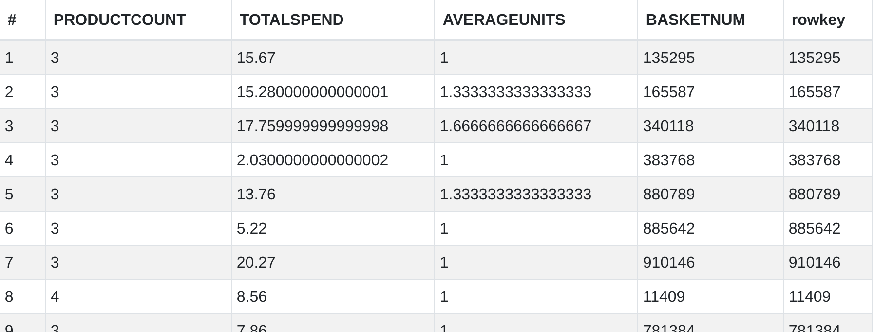
Example 1: Basic Aggregation
This is an example of a simple query that performs some aggregations and filters the results both before and after the grouping.
Query
select
    basketnum,
    count(*) as ProductCount,
    sum(spend) as TotalSpend,
    avg(units) as AverageUnits
from transactions
where storer = 'CENTRAL'
group by basketnum
having count(*) > 2
Output
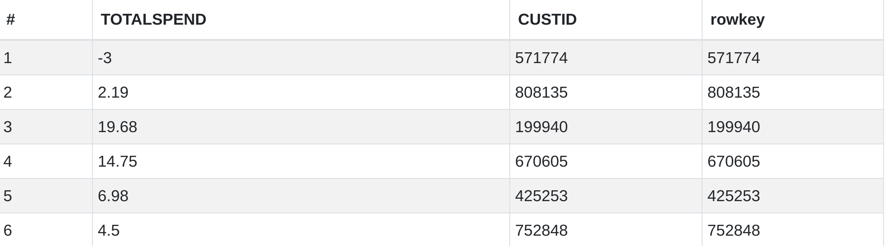
Example 2: Basic Join
This query uses a join to compute the total amount spent by each customer.
Query
select
    custid,
    sum(spend) as TotalSpend
from transactions t
inner join customers c
    on t.basketnum = c.basketnum
group by custid
Output
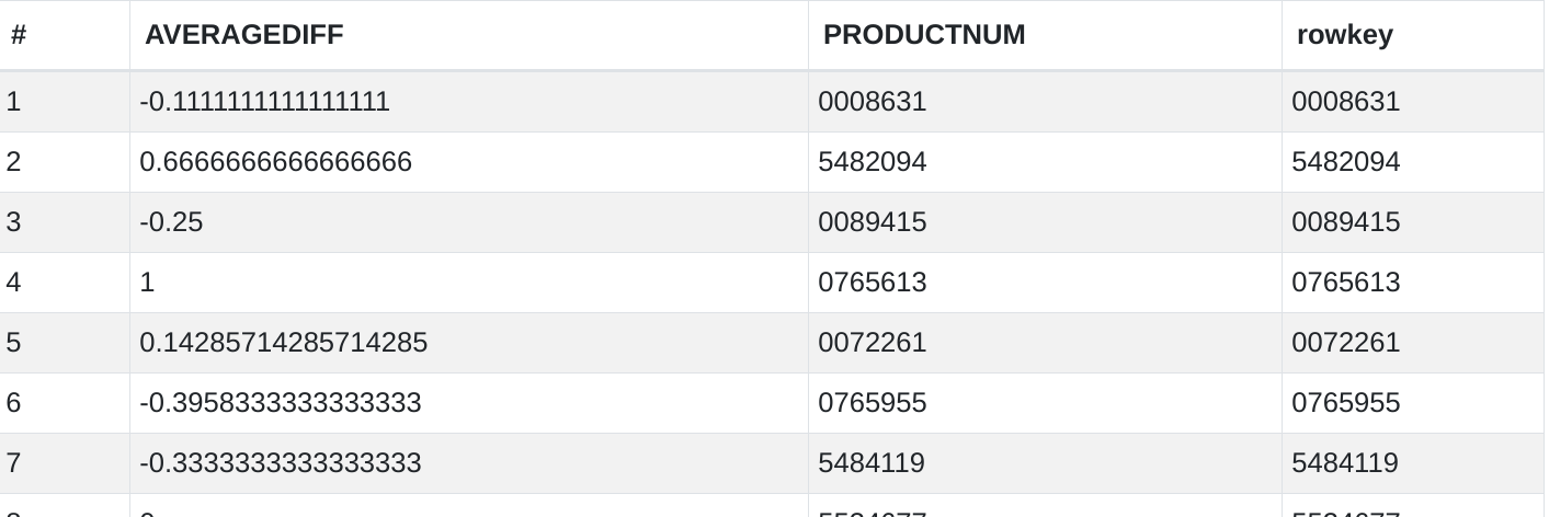
Example 3: Subquery
Like in a relational database, the output from one query can be used as the input in another one. The following query investigates differences in quantity purchased per transaction for each productnum between the CENTRAL and SOUTH stores.
Query
select
    central_products.productnum,
    avg(central_products.units - south_products.units) as AverageDiff
from
(
    select productnum, units
    from transactions
    where storer = 'CENTRAL'
) as central_products
inner join
(
    select productnum, units
    from transactions
    where storer = 'SOUTH'
) as south_products
on central_products.productnum = south_products.productnum
group by 1;
Output
Example 4: Common Table Expression
Instead of placing subqueries inline, they can also be defined ahead of time using common table expressions. For instance, the previous example could be rewritten as the following query:
Query
with central_products as (
    select productnum, units
    from transactions
    where storer = 'CENTRAL'
), south_products as (
    select productnum, units
    from transactions
    where storer = 'SOUTH'
)
select
    central_products.productnum,
    avg(central_products.units - south_products.units) as AverageDiff
from central_products
inner join south_products
    on central_products.productnum = south_products.productnum
group by 1;
Output
The output is the same as Example 3
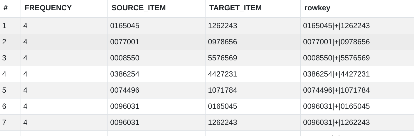
Example 5: Self-join
Burroughs supports selj-joins, something that is not inherently supported by KsqlDB. The below example uses a self-join to find the frequency with with certain combinations of items appear in the same basket.
Query
with pairs as (
    select
        it1.productnum as source_item,
        it2.productnum as target_item
    from transactions it1
    inner join transactions it2
        on it1.basketnum = it2.basketnum
        and it1.productnum < it2.productnum
    where
        it1.units > 0
        and it2.units > 0
)
select
    source_item,
    target_item,
count(1) as frequency
from pairs
group by 1,2
having count(1) > 2;
Output
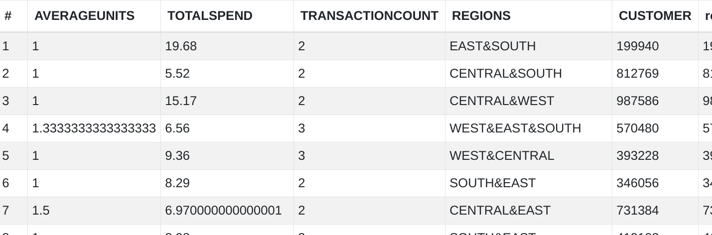
Example 6: Group_Concat
group_concat, as described in the previous section, is an aggregate function that appends all of the values for a given field in each group together into one long string. The user can specify the separator to use between values as well as whether to include duplicates. The below query gets a list of all of the locations a customer has shopped at, in addition to other summary statistics.
Query
select
    custid as Customer,
    avg(units) as AverageUnits,
    sum(spend) as TotalSpend,
    count(*) as TransactionCount,
    group_concat(distinct storer, '&') as Regions
from transactions t
left join customers c
    on t.basketnum = c.basketnum
group by 1;
Output
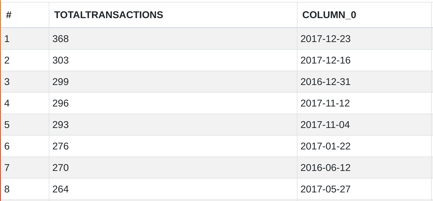
Example 7: Date Manipulation
Burroughs, like its dependencies Avro and KsqlDB, does not support any kind of date data type. Instead, dates must be stored as integers representing the number of days since the epoch. Such dates are not human readable, so Burroughs provides the ability to turn those into normal date strings using the cast function as shown in the following query which counts the total number of transactions that occur on each day.
Query
select
    cast("Date" as Date),
    count(*) as TotalTransactions
from transactions
group by 1;
Note: if date is a column name, it must be surrounded by double quotes because date is a keyword in SQL
Output
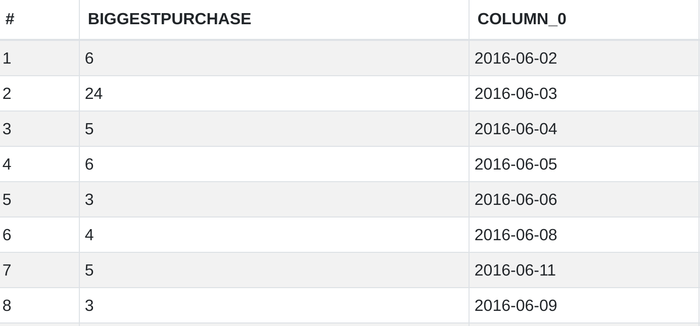
You can also use the cast function to transform a literal date to the proper integer representation for comparison, like in the following query, which finds largest purchase in terms of quantity for each date after June 1, 2016.
Query
select
    max(units) as BiggestPurchase,
    cast("Date" as Date) from transactions
where "Date" > CAST('2016-06-01' as date)
group by 2;
Output
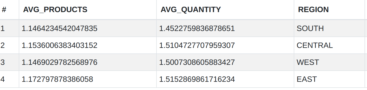
Example 8: Multiple Group By Clauses
The following query is an example of performing aggregations in multiple stages using common table expressions. Note that it would be cleaner to group by storer in addition to basketnum in the inner query, but this is not possible because Burroughs does not allow multiple fields in the group by of a CTE. Instead, the function earliest_by_offset is used to include the region, assuming that each basket number belongs to only one region.
Query
with raw as (
    select
        earliest_by_offset(store_r) as region,
        basketnum,
        count(1) as num_products,
        sum(units) as total_quantity
    from transactions
    group by 2
)
select
    region,
    avg(num_products) as avg_products,
    avg(total_quantity) as avg_quantity
from raw
group by 1;
Output