PERiLS 2022#
author: Hamid Ali Syed
date: May 12, 2023
import warnings
warnings.filterwarnings("ignore")
import pandas as pd
import hvplot.pandas
import geoviews as gv
import numpy as np
import matplotlib.pyplot as plt
import cartopy.crs as ccrs
from IPython.display import display
import geopandas as gpd
import shapely.geometry as sgeom
from cartopy.geodesic import Geodesic
import urllib.request
from pathlib import Path
import nearest_nexrad as nrnx
# This is to find nearest nexrad radars, and associated lats,lons
file_name = "nearest_nexrad.py"
url = "https://raw.githubusercontent.com/syedhamidali/test_scripts/master/nearest_nexrad.py"
if not Path(file_name).is_file():
urllib.request.urlretrieve(url, file_name)
print(nrnx.get_nexrad_location("KGWX"))
(33.89667, -88.32889, 476)
df = pd.read_excel("Data_availability_PERiLS.xlsx")
df.drop([9, 10, 11], inplace=True)
df.reset_index(drop=True, inplace=True)
df
| Instrument | Lon | Lat | Range[m] | IOP | Start_Time | End_Time | |
|---|---|---|---|---|---|---|---|
| 0 | COW1 | -87.946000 | 32.810980 | 88443.41 | IOP1 | 2022-03-22 17:04:44 | 2022-03-22 23:03:40 |
| 1 | DOW7 | -88.171700 | 32.710800 | 74960.42 | IOP1 | 2022-03-22 17:59:03 | 2022-03-22 23:37:13 |
| 2 | DOW8 | -88.436500 | 33.262500 | 58545.50 | IOP1 | 2022-03-22 20:02:00 | 2022-03-22 21:08:50 |
| 3 | COW1 | -88.548200 | 33.606340 | 88443.41 | IOP2 | 2022-03-30 15:52:26 | 2022-03-31 02:18:40 |
| 4 | DOW7 | -88.608500 | 33.485000 | 74960.42 | IOP2 | 2022-03-30 18:57:33 | 2022-03-31 02:19:07 |
| 5 | DOW8 | -88.662700 | 33.723800 | 73529.96 | IOP2 | 2022-03-30 21:42:12 | 2022-03-31 02:20:11 |
| 6 | COW1 | -86.544500 | 32.269600 | 88443.41 | IOP3 | 2022-04-05 12:32:48 | 2022-04-05 17:28:42 |
| 7 | DOW7 | -86.679100 | 32.428000 | 74960.42 | IOP3 | 2022-04-05 13:01:09 | 2022-04-05 16:24:53 |
| 8 | DOW8 | -86.430200 | 32.197800 | 58545.50 | IOP3 | 2022-04-05 14:39:27 | 2022-04-05 17:29:50 |
| 9 | UAHM | -88.495400 | 33.132500 | 50000.00 | IOP1 | 2022-03-22 22:34:17 | 2022-04-13 20:22:14 |
| 10 | UAHM | -88.712067 | 33.840030 | 99750.00 | IOP2 | 2022-03-30 15:13:12 | 2022-03-31 01:42:02 |
| 11 | NOXP | -88.495216 | 33.132534 | 74962.00 | IOP2 | 2022-03-30 18:29:28 | 2022-03-31 01:34:18 |
| 12 | SMARTR1 | -88.345871 | 32.888432 | 98975.00 | IOP1 | 2022-03-22 16:05:24 | 2022-03-22 21:17:49 |
| 13 | SMARTR2 | -88.570110 | 33.213134 | 81900.00 | IOP1 | 2022-03-22 15:49:30 | 2022-03-22 22:48:37 |
| 14 | SMARTR2 | -88.484060 | 33.346680 | 82950.00 | IOP2 | 2022-03-30 19:11:36 | 2022-03-31 02:27:34 |
def calculate_centroid(df):
centroid_lat = df['Lat'].mean()
centroid_lon = df['Lon'].mean()
return centroid_lat, centroid_lon
def draw_circle_on_map(df):
gd = Geodesic()
geoms = []
for _, row in df.iterrows():
lon, lat = row['Lon'], row['Lat']
radius = row['Range[m]']
cp = gd.circle(lon=lon, lat=lat, radius=radius)
geoms.append(sgeom.Polygon(cp))
gdf = gpd.GeoDataFrame(df, geometry=geoms)
gdf.crs = "EPSG:4326" # set the CRS
return gdf
def draw_circle_on_map_for_nexrad(df):
gd = Geodesic()
geoms = []
for _, row in df.iterrows():
lon, lat = row['lon'], row['lat']
if row['ID'].startswith('T'):
radius = 90e3
else:
radius = 250e3
cp = gd.circle(lon=lon, lat=lat, radius=radius)
geoms.append(sgeom.Polygon(cp))
gdf = gpd.GeoDataFrame(df, geometry=geoms)
gdf.crs = "EPSG:4326" # set the CRS
return gdf
def create_plot(switch):
gdf = draw_circle_on_map(df)
# Define the data based on the switch variable
if switch == 'IOP1':
data = gdf[gdf['IOP'] == 'IOP1']
elif switch == 'IOP2':
data = gdf[gdf['IOP'] == 'IOP2']
elif switch == 'IOP3':
data = gdf[gdf['IOP'] == 'IOP3']
else:
data = gdf
centroid_lat, centroid_lon = calculate_centroid(data)
sites = nrnx.nearest_sites(centroid_lat, centroid_lon, 4).reset_index(drop=True)
gsites = draw_circle_on_map_for_nexrad(sites)
# Define the colormap for instrument colors
instrument_colors = {'COW1': 'red', 'DOW7': 'blue', 'DOW8': 'green',
'UAHM': 'orange', 'NOXP': 'purple', 'SMARTR1': 'cyan',
'SMARTR2': 'magenta'}
# Create a color column based on the Instrument column
data['Color'] = data['Instrument'].map(instrument_colors)
# Define the point plot based on the data
points = data.hvplot.points(x='Lon', y='Lat', geo=True, color='Color',
alpha=0.7, coastline=True,
frame_height=800, frame_width=650,
hover_cols=['Instrument', 'Range[m]', 'IOP', 'Start_Time', 'End_Time'])
# Define the circle plot based on the data
circles = gv.Polygons(data=data.geometry).opts(fill_alpha=0.2,
xlabel='Lon˚E', ylabel='Lat˚N',
frame_height=800, frame_width=650)
# Define the point plot for the gsites data
points_nex = gsites.hvplot.points(x='lon', y='lat', geo=True, color='k',
alpha=0.7, hover_cols=['ID'],
coastline=True,
tiles='OpenTopoMap',
frame_height=800, frame_width=650)
# Define the circle plot for the gsites data
circles_nex = gv.Polygons(data=gsites.geometry).opts(color='w', fill_alpha=0.2,
xlabel='Lon˚E', ylabel='Lat˚N',
frame_height=800, frame_width=650)
# Overlay the circle plot on top of the point plot
plot = points_nex * circles_nex * points * circles
# Save the figure as HTML
html_path = f"plot_{switch}.html"
hvplot.save(plot, html_path)
return plot
create_plot('IOP2')
snd = pd.read_excel("SONDE_UIUC.xlsx")
snd
| IOP | Date | Vehicle ID | Sonde ID | Launch Time (UTC) | Latitude\n(degrees) | Latitude - Sonde GPS\n(degrees) | Latitude FINAL\n(degrees) | Longitude\n(degrees) | Longitude - Sonde GPS\n(degrees) | Longitude FINAL\n(degrees) | Altitude\n(m MSL) | Altitude - USGS NED\n(m MSL) | Altitude FINAL\n(m MSL) | |
|---|---|---|---|---|---|---|---|---|---|---|---|---|---|---|
| 0 | 1.0 | 20220322.0 | SONDE1 | 18043739 | 18:03:43 | 32.91079 | 32.9108 | 32.91080 | -88.29812 | -88.29814 | -88.29815 | 0 | 49 | 49 |
| 1 | NaN | NaN | NaN | 18047099 | 19:15:54 | 32.91078 | 32.9108 | 32.91080 | -88.29812 | -88.29815 | -88.29815 | 0 | 49 | 49 |
| 2 | NaN | NaN | NaN | 18043171 | 19:56:52 | 32.91080 | 32.9108 | 32.91080 | -88.29816 | -88.29814 | -88.29815 | 0 | 49 | 49 |
| 3 | NaN | NaN | NaN | 18043798 | 20:41:29 | 32.91079 | 32.9108 | 32.91080 | -88.29813 | -88.29815 | -88.29815 | 0 | 49 | 49 |
| 4 | NaN | NaN | SONDE2 | 18047276 | 18:11:32 | 32.70832 | 32.7083 | 32.70835 | -88.20456 | -88.20450 | -88.20430 | 0 | 62 | 62 |
| ... | ... | ... | ... | ... | ... | ... | ... | ... | ... | ... | ... | ... | ... | ... |
| 103 | NaN | NaN | NaN | 21059195 | 20:43:54 | 36.11820 | 36.1186 | 36.11830 | -90.16840 | -90.16836 | -90.16840 | 130 | 78 | 78 |
| 104 | NaN | NaN | SONDE5 | 21058975 | 19:14:03 | 36.49007 | 36.4901 | 36.49010 | -90.01672 | -90.01671 | -90.01671 | 97 | 87 | 87 |
| 105 | NaN | NaN | NaN | 21058928 | 20:01:53 | 36.49018 | 36.4902 | 36.49010 | -90.01678 | -90.01671 | -90.01671 | 97 | 87 | 87 |
| 106 | NaN | NaN | NaN | 21059115 | 20:32:37 | 36.49085 | 36.4908 | 36.49080 | -90.01636 | -90.01631 | -90.01630 | 97 | 87 | 87 |
| 107 | NaN | NaN | NaN | 21051157 | 21:00:18 | 36.49086 | 36.4909 | 36.49080 | -90.01633 | -90.01630 | -90.01630 | 97 | 87 | 87 |
108 rows × 14 columns
snd = snd[['IOP','Date','Launch Time (UTC)','Vehicle ID',
'Latitude FINAL\n(degrees)','Longitude FINAL\n(degrees)',
'Altitude FINAL\n(m MSL)']]
def fill_nans(df, columns):
values = {} # Initialize a dictionary to store the non-NaN values for each column
for column in columns:
values[column] = None # Initialize the value for each column
for idx, row in df.iterrows():
if not pd.isnull(row[column]): # Check if the value is not NaN
values[column] = row[column] # Update the value with the non-NaN value
df.at[idx, column] = values[column] # Fill NaN values with the current value
if column == 'IOP':
df[column] = df[column].replace({1.0: 'IOP1', 2.0: 'IOP2', 3.0: 'IOP3', 4.0: 'IOP4'})
elif column == 'Date':
df[column] = pd.to_datetime(df[column], format='%Y%m%d')
# Rename columns
df.rename(columns={'Latitude FINAL\n(degrees)': 'lat',
'Longitude FINAL\n(degrees)': 'lon',
'Launch Time (UTC)': 'time',
'Altitude FINAL\n(m MSL)':'alt'},
inplace=True)
return df
def create_datetime_column(df):
df['datetime'] = pd.to_datetime(df['Date'].astype(str) + ' ' + df['time'].astype(str))
return df
filled_snd = fill_nans(snd, ['IOP', 'Date', 'Vehicle ID'])
filled_snd = create_datetime_column(filled_snd)
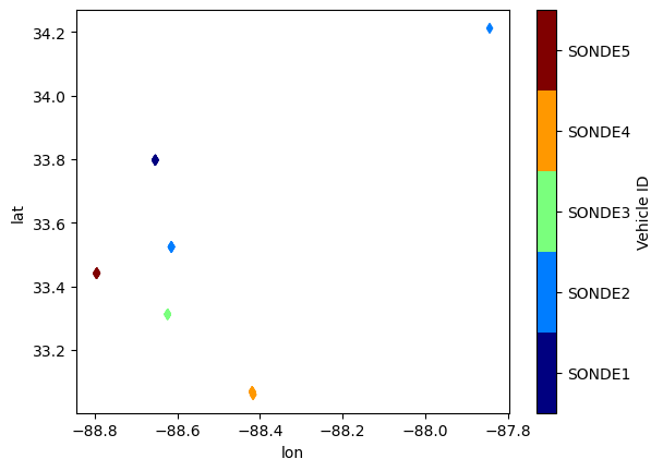
filled_snd['Vehicle ID'] = pd.Categorical(filled_snd['Vehicle ID'])
filled_snd[filled_snd['IOP']=='IOP2'].plot.scatter(x='lon', y='lat', c='Vehicle ID', cmap='jet', marker='d')
<AxesSubplot:xlabel='lon', ylabel='lat'>
def plot_domain_with_snd(switch):
gdf = draw_circle_on_map(df)
# Define the data based on the switch variable
if switch in ['IOP1', 'IOP2', 'IOP3']:
data = gdf[gdf['IOP'] == switch]
else:
data = gdf
centroid_lat, centroid_lon = calculate_centroid(data)
sites = nrnx.nearest_sites(centroid_lat, centroid_lon, 4).reset_index(drop=True)
gsites = draw_circle_on_map_for_nexrad(sites)
# Convert data to a GeoDataFrame
data = gpd.GeoDataFrame(data, geometry='geometry')
# Define the point plot based on the data
points = data.hvplot.points(x='Lon', y='Lat', geo=True, marker='o', color='r',
alpha=0.7, coastline=True,
frame_height=800, frame_width=650,
hover_cols=['Instrument', 'Range[m]', 'IOP', 'Start_Time', 'End_Time'])
# Define the circle plot based on the data
circles = gv.Polygons(data=data).opts(color='gray', fill_alpha=0.2,
xlabel='Lon', ylabel='Lat',
frame_height=800, frame_width=650)
# Define the point plot for the gsites data
points_nex = gsites.hvplot.points(x='lon', y='lat', geo=True, color='k',
alpha=0.7, hover_cols=['ID'],
coastline=True,
tiles='OpenTopoMap',
frame_height=800, frame_width=650)
# Define the circle plot for the gsites data
circles_nex = gv.Polygons(data=gsites.geometry).opts(color='w', fill_alpha=0.2,
xlabel='Lon', ylabel='Lat',
frame_height=800, frame_width=650)
# Overlay the circle plot on top of the point plot
plot = points_nex * circles_nex * points * circles
# Filter filled_snd based on switch
filled_snd_filtered = filled_snd[filled_snd['IOP'] == switch]
# Convert filled_snd to hvPlot
hv_snd = filled_snd_filtered.hvplot.points(x='lon', y='lat', c='Vehicle ID', marker='d',
geo=True, hover_cols=['Vehicle ID', 'datetime', 'alt'],
size=100)
# Overlay filled_snd plot on top of the existing plot
plot = plot * hv_snd
# Save the figure as HTML
html_path = f"plot_domain_radsnd_{switch}.html"
hvplot.save(plot, html_path)
return plot
plot_domain_with_snd("IOP2")
plot_domain_with_snd("IOP1")
plot_domain_with_snd("IOP3")